|
|
||
|
Examples
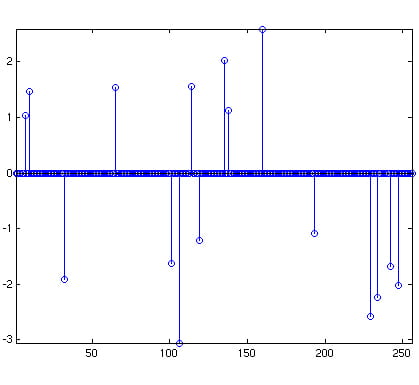
The central idea in compressive sampling is that the number of samples As a concrete example, suppose that f is a discrete signal (of length
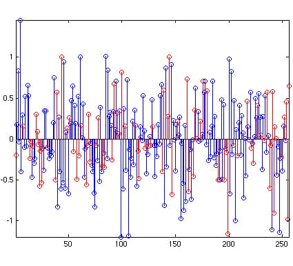
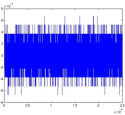
How many time-domain samples do we need Now suppose that we are given only 80 samples. Below is a plot
Of course, we will not be able to “fill
|
||
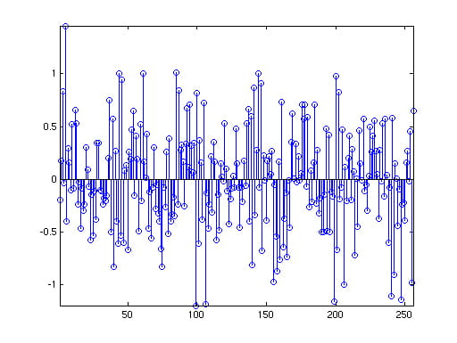
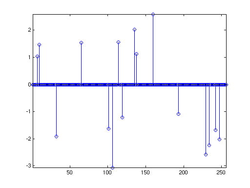 Recovered signal, frequency domain
|
||
| In general, if there are B sinusoids in the signal, we will be able to recover using L1 minimization from on the order of B log N samples (see the “Robust Uncertainty Principles…” paper for a full exposition).
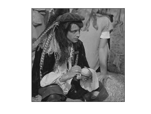
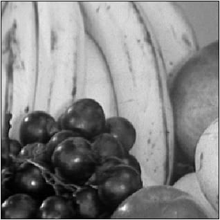
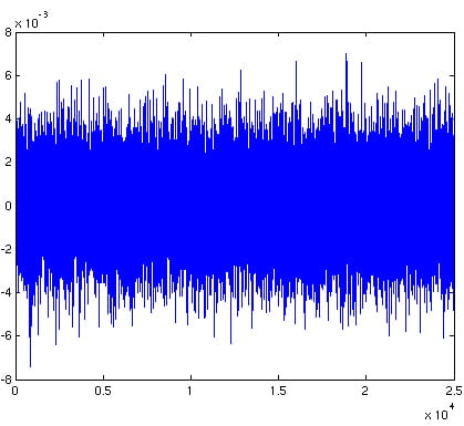
The framework is easily extended to more general types of measurements Here is an example. The 1 megapixel image below has a perfectly Instead of observing this image directly, say we took 100,000 “random
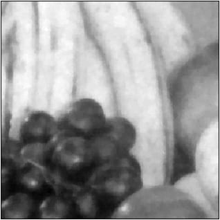
The lesson here is that the number of measurements needed to acquire this In the “real world”, signals and images are not perfectly sparse, and Another example in imaging is given below: we observe 25,000 random measurements |
||
 |
 |
|
|
65k pixel image
|
25k random measurements
|
|
 |
 |
|
|
quantized measurements
|
recovered image
|
|
|
The L1-MAGIC package includes MATLAB code that solves these (and |
||